Interactive App

gui/TemporalMapperApp.m is a point-and-click alternative to the scripted pipeline in the Quickstart — load data, pick variables, set parameters, and view the resulting network without writing any code. It wraps exactly the same two-step pipeline (tknndigraph → filtergraph) and the same plotting functions (plottmgraph/plotgraphtcm) described elsewhere in these docs, so everything in Concepts about what the parameters mean still applies.

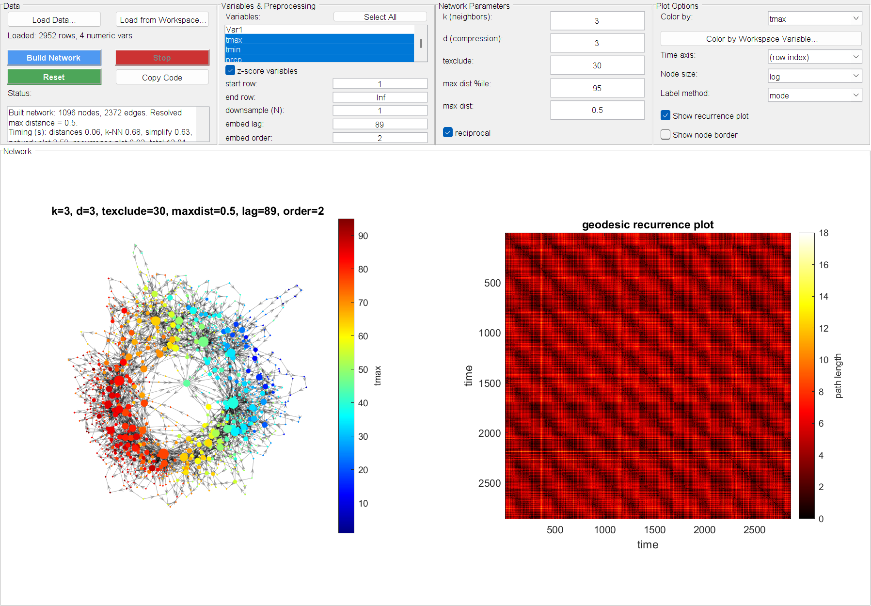
The same East Lansing weather dataset and parameters as the Quickstart, built through the app instead of the command line.

Launch it

addpath("tmapper_tools/")
addpath("gui/")
app = TemporalMapperApp;

Layout

The window is split into two parts: four Setup panels across the top, and the Network/recurrence plots filling the rest of the window.

Data

Load a data file (.csv/.txt, read with readtable) or a table/numeric matrix already sitting in your base workspace. Only numeric columns are offered as build variables. This panel also holds Build Network, Stop (cancels an in-progress build — see below), Reset (restores every parameter to its default, but leaves your loaded data and variable selection alone), Copy Code, Export... (see below), and a live Status box with per-step timing once a build finishes.

Variables & Preprocessing

• Variables — the numeric columns to build the network from (⌘/Ctrl/Shift-click for multiple; Select All as a shortcut). A leading unnamed row-index column is dropped automatically — see below.
• z-score variables — on by default; see the Quickstart's note on why.
• start row / end row — restrict the build to a sub-range of the loaded data. end row = Inf means "the last row."
• time index — which column says who is temporally adjacent. Defaults to row order; pick a column for data with real breaks (separate sessions/trials). See below.
• downsample (N) — keep every Nth row. A moving-average lowpass is applied first so this doesn't alias high-frequency content into spurious low-frequency structure — see below.
• embed lag / embed order — optional delay embedding; order 1 (default) skips it.

Network Parameters

The four tknndigraph/filtergraph parameters explained in the Quickstart and Concepts: k, d (labeled "compression"), texclude, the two max dist cutoffs, and reciprocal.

Plot Options

Color/time axis variable, node size mode, label method, and whether to show the recurrence plot / a node-border scatter overlay. Changing any of these re-renders the existing network instead of rebuilding it — cheap, and safe to click through freely once a build has completed.

Colouring by a category

Text columns (condition, trial, behavioural state) are offered under Color by. They are treated as purely nominal: labels map to integer codes, the colour axis is pinned so each category owns an equal band (so a category keeps its colour between builds), and mean/median are withdrawn from Label method — averaging codes 1 and 3 gives code 2, which is a different category, not an average of two. Pair them with a qualitative colormap.

They stay out of Variables and Time axis: distances and a time axis both need an order that nominal labels do not have.

Colormap

jet by default, matching plottmgraph's own default. lines, prism and colorcube are qualitative — adjacent entries are unrelated rather than a ramp — which is what discrete labels need; the rest are continuous.

Date columns

readtable turns a date column into datetime automatically, and those columns are offered for Color by and Time axis — so the GUI can reproduce tmapper_demo.m's own t = dat.Date axis, with the recurrence plot labelled in real dates rather than row numbers.

They stay out of Variables, though: distances need real numbers. For colouring, a date is converted with datenum (a colormap needs numbers, and plottmgraph calls isnan on the colour variable, which errors on datetime); the time axis keeps the datetime as-is, since imagesc takes it natively.

Missing data and downsampling

Several things the scripted pipeline leaves to you are handled automatically here:

Oversized row ranges are refused, not attempted

Rather than thrash or exhaust memory, the app refuses up front, before any of the expensive work, and tells you the figure and how to fix it. The count is taken after decimation, so raising downsample (N) is a real fix rather than a way around the check.

The budget is half this machine's physical RAM (clamped to 2–32 GB), not a fixed number — half is a defensible share for one analysis app, and using total rather than currently available keeps the limit stable between runs. If the platform can't be queried it falls back to 4 GB.

Neither the graph build nor the simplification sets that ceiling any more. The build runs on tknndigraph's lowMemory path, which computes distances a block of rows at a time and never allocates an N×N array; filtergraph thresholds geodesics by sparse reachability rather than materialising them. Both are roughly flat in N.

What remains is the recurrence plot, which is genuinely an N×N image of geodesic distances between time points — the feature itself, not waste. So the ceiling depends on whether you are showing it, and unchecking it is a real way to go bigger:

Show recurrence plot	Peak memory	Scaling
on	4.08 GB at 20 000 points	quadratic — binds first
off	2.10 / 2.13 / 2.14 GB at 20 000 / 40 000 / 56 000	flat

With it hidden, memory stops being the constraint entirely, so the guard switches to limiting on time (15 minutes) and says which of the two you actually hit. On a 64 GB machine that works out at roughly 62 000 points with the recurrence plot and 130 000 without.

A stray row-index column is dropped

Writing a CSV without suppressing the index leaves an unnamed first column, which readtable names Var1. It is just a monotonic ramp, so leaving it selectable — and selected by default — would silently dominate the distance computation. It is dropped on load and the status area says so.

Var1 is a weaker signal than it looks, since MATLAB also auto-names every column of a genuinely header-less file, so the check additionally requires that some other column is properly named and that the column really does look like a row index (numeric and strictly increasing). A Var1 holding real data is kept.

Missing data is handled, not ignored

A missing value in any selected variable is never passed through to the pipeline — an unremoved NaN would poison the entire distance matrix without any visible error. Calling tknndigraph/plottmgraph directly on unclean data still raises an error, per the usual rmmissing-first convention.

At downsample (N) = 1 a row with any missing selected variable is dropped, leaving a real gap in time. When downsampling, each kept sample is an average over its window and that average simply skips missing inputs — so an isolated NaN costs no sample at all, and only a sample whose entire window is missing is dropped. The status area reports the count either way.

Downsampling anti-aliases first

Setting downsample (N) > 1 applies a moving-average lowpass over a window of size N before striding, rather than naively picking every Nth raw row.

Decimation runs on the original row grid, never on the rows left after missing-data removal. Striding the survivors would slide every later sample off the true time grid, inventing gaps between samples that were in fact evenly spaced.

Supplying your own time index

By default tidx comes from row position, which is right for a single continuous recording. For data with genuine breaks — separate sessions or trials — pick a time index column instead, and the breaks survive as breaks rather than being bridged.

The unit is the smallest step between kept samples, so any larger step is a real gap. The column must be strictly increasing and on a regular grid (every step a whole multiple of the smallest); a genuinely irregular index has no integer grid to sit on and is refused rather than silently distorted. Numeric and datetime columns both work.

Real gaps stay gaps in time

tknndigraph's tidx argument is what tells the pipeline which samples are temporally adjacent — it links two points only when their tidx differs by exactly 1. The app derives tidx from elapsed position rather than array position, so a genuine break in the data (a dropped row, or a restricted row range) leaves a jump and no temporal edge is fabricated across it.

Stop cancels between, not mid-stage

Stop requests cancellation, but MATLAB callbacks run synchronously, so it only takes effect at the boundary between stages (distances → k-NN graph → simplify) — not mid-computation within one. For a very slow single stage (usually the distance/k-NN step on a large dataset), it may take a moment to actually stop.

Export

Export... asks for a folder and writes everything needed to carry the result into downstream analysis or a paper:

File	What it is
network.png	the attractor transition network, at 200 dpi
recurrence.png	the geodesic recurrence plot (only when it is shown)
timeline.csv	one row per retained time point: tidx, source_row, node, plus the chosen colour/time columns
params.json	full provenance — every preprocessing and network setting, the resolved maxNeighborDist, and the resulting network's size
reproduce.m	the same standalone script Copy Code puts on the clipboard

timeline.csv is the one that matters most: it is the join-back table saying which attractor the system was in at each time point, which is what dwell-time, transition-rate and occupancy analyses actually need — and the one thing that cannot be recovered from the figures.

The figures are written from the axes rather than the window, so you get just the plot, not a screenshot of the whole GUI.

params.json records the build, not the controls

Every value in it comes from the build that produced these figures, so changing a field after building and then exporting still describes what you are actually looking at.

Copy Code

Copy Code puts a complete, standalone script on the clipboard that reproduces the current build — including the data-loading line if you loaded a file — using the exact resolved parameters shown in the app. This is the bridge back to scripting: prototype interactively here, then paste the generated code into your own analysis once you have parameters you like.

What's next

• Concepts — what the network's nodes, edges, and loops mean.
• Quickstart — the same pipeline, scripted end to end.